Disclaimer: This blog and all associated research are part of my personal independent study. All hardware, software, and infrastructure are personally owned and funded. No employer resources, property, or proprietary information are used in any part of this work. All opinions and content are my own.
This post continues from Part 1 where the Jetson Orin Nano was installed and configured.
Before running real experiments, I want to confirm the ML stack is fully working:
- Python runs correctly
- PyTorch is installed and functional
- CUDA is available and the GPU is visible
- A training loop runs end-to-end on the GPU
If you’re coming from a malware analysis or reverse engineering background and haven’t worked with machine learning before, don’t worry — I’ll explain each concept as we go. The code is simple, and the goal here is just to verify the environment, not to build anything complex yet.
All tests below were run inside the Jupyter container on the Jetson.
Setting Up the Notebook
Start the Jupyter container from Part 1 if it isn’t already running:
docker start jetson-jupyter
docker logs jetson-jupyter 2>&1 | grep token
Open JupyterLab in a browser and create a new notebook called env_check.ipynb. A Jupyter notebook lets you run Python code in individual cells and see results immediately — similar to running commands one at a time in a Python REPL, but with the ability to save, reorder, and re-run them.
Cell 1 — System Info
import sys
import platform
import os

print("Python:", sys.version)
print("Platform:", platform.platform())
print("Machine:", platform.machine())
print("Working dir:", os.getcwd())
This cell collects basic runtime information about the Python interpreter and the host system. On the Jetson, platform.machine() should return aarch64, confirming we’re running on ARM64 architecture rather than the more common x86_64 found on desktop/server machines.
Why this matters for malware research: Most malware analysis tooling (IDA, Ghidra, YARA, etc.) runs on x86_64. The Jetson is ARM — so not every Python package ships pre-built binaries for this platform. Some will need to be compiled from source or installed from NVIDIA’s custom repositories. Knowing the architecture upfront saves debugging time when a pip install fails later.
Checking the working directory also confirms that the Docker volume mount (-v ~/workspace:/workspace) from Part 1 is correctly mapped, so files you create inside the container persist on the host.
Cell 2 — NumPy
import numpy as np

print("NumPy version:", np.__version__)
print(np.arange(10))
What is NumPy? NumPy is a Python library for working with arrays of numbers efficiently. If you’ve ever written a YARA rule that scans byte sequences, or a script that processes PE header fields — NumPy does the same kind of bulk data manipulation, but optimized for millions of values at once. Nearly every ML library (including PyTorch) depends on it.
np.arange(10) creates a simple array [0, 1, 2, 3, 4, 5, 6, 7, 8, 9]. It’s trivial, but it exercises NumPy’s core array allocation and verifies that the underlying math libraries (BLAS/LAPACK) are correctly installed on ARM. These are the same libraries that power the matrix operations in every ML model.
Cell 3 — PyTorch and CUDA
import torch

print("Torch version:", torch.__version__)
print("CUDA available:", torch.cuda.is_available())
print("CUDA version:", torch.version.cuda)
What is PyTorch? PyTorch is a machine learning framework — think of it as a toolkit for building and training models. You define a model (a mathematical function with tunable parameters), feed it data, and PyTorch handles the math to automatically adjust those parameters so the model gets better at its task. It’s what we’ll eventually use to train malware classifiers.
What is CUDA? CUDA is NVIDIA’s programming interface for running computations on the GPU instead of the CPU. GPUs have thousands of small cores that can perform many operations in parallel — this makes them dramatically faster for the matrix math that ML models rely on. Without CUDA, training would run on the CPU and be orders of magnitude slower.
This is the most critical check. torch.cuda.is_available() returns True only if:
- PyTorch was compiled with CUDA support (the
dustynv/l4t-pytorchcontainer handles this) - The NVIDIA driver is accessible from inside the container (
--runtime nvidia) - A compatible GPU is detected
If CUDA available shows False, the most common cause is that the container wasn’t started with --runtime nvidia. Other causes include driver version mismatches between the host JetPack and the container’s CUDA toolkit. The torch.version.cuda string (e.g., 12.2) should match the JetPack CUDA version shown by nvcc --version on the host.
Cell 4 — GPU Detection
if torch.cuda.is_available():
    print("GPU count:", torch.cuda.device_count())
    for i in range(torch.cuda.device_count()):
        print(f"  [{i}] {torch.cuda.get_device_name(i)}")
else:
    print("GPU not detected")
torch.cuda.device_count() returns the number of CUDA-capable GPUs visible to PyTorch. The Jetson Orin Nano has a single integrated GPU, so this should return 1.
Key difference from desktop GPUs: Unlike a discrete GPU (like an RTX 4090) that has its own dedicated video memory (VRAM), the Jetson’s GPU shares unified memory with the CPU — they both use the same physical RAM. On the Orin Nano with 8GB total, expect roughly 4-5GB usable for ML work after the OS and container overhead. This is a constraint we’ll need to keep in mind when choosing model sizes and batch sizes for malware classification experiments.
get_device_name() returns the GPU identifier string, which is useful for logging. If you later run the same notebook on a different machine, the name change will be immediately visible in the output — important for keeping experiments reproducible.
Cell 5 — Tensor Operations on GPU
device = "cuda" if torch.cuda.is_available() else "cpu"

x = torch.randn(1024, 1024, device=device)
y = torch.randn(1024, 1024, device=device)

z = (x @ y).mean()
print("Device:", device)
print("Result:", z.item())
What is a tensor? A tensor is just a multi-dimensional array of numbers. A 1D tensor is a list, a 2D tensor is a table/matrix, a 3D tensor is a stack of tables, and so on. In malware ML, your input data will typically be tensors — for example, a batch of 100 malware samples each represented as a vector of 256 features would be a tensor with shape (100, 256).
Here’s what each line does:
torch.randn(1024, 1024, device=device)— creates a 1024x1024 matrix filled with random numbers, allocated directly on the GPU. Thedevice="cuda"part is key — without it, the data lives on CPU RAM and would need to be copied to the GPU before the GPU can work with it.x @ y— matrix multiplication (same astorch.matmul(x, y)). This is the fundamental operation behind ML models. When a model makes a prediction, it’s essentially multiplying your input data by learned weight matrices. A 1024x1024 matmul involves about 2 billion arithmetic operations..mean()— averages all values in the result down to a single number..item()— copies that single number from GPU memory back to the CPU so Python can print it.
The actual numeric result doesn’t matter (it should be close to zero since we’re averaging random numbers). What matters is that the operation completes without CUDA errors — proving the GPU can allocate memory, compute, and return results.
Cell 6 — GPU Performance Check
import time

device = "cuda" if torch.cuda.is_available() else "cpu"

x = torch.randn(2048, 2048, device=device)
y = torch.randn(2048, 2048, device=device)

# Warm-up runs
for _ in range(3):
    _ = (x @ y).sum()
torch.cuda.synchronize()

t0 = time.time()
_ = (x @ y).sum()
torch.cuda.synchronize()
t1 = time.time()

print(f"2048x2048 matmul: {t1 - t0:.4f}s")
This cell benchmarks the GPU, but GPU benchmarking is trickier than CPU benchmarking. Here’s why:
CUDA operations are asynchronous. When Python runs x @ y, it doesn’t wait for the GPU to finish — it just sends the instruction and moves on immediately. This is like dropping a job in a queue. So if you just wrap time.time() around the operation, you’d measure how long it took to submit the job (microseconds), not how long the GPU took to complete it.
Two techniques fix this:
-
Warm-up runs: The very first GPU operation in a session triggers one-time setup — compiling CUDA kernels, allocating memory pools, initializing the GPU scheduler. The 3 warm-up iterations absorb these startup costs so they don’t inflate the benchmark.
-
torch.cuda.synchronize(): This tells Python to wait until the GPU finishes all pending work before continuing. By calling it before starting the timer and after the operation, we ensuret1 - t0measures the actual GPU compute time.
A 2048x2048 matmul involves about 17 billion arithmetic operations. On the Orin Nano, expect this to complete in a few milliseconds. This gives you a performance baseline — useful later when you want to compare how long it takes to run inference on a batch of malware samples.
Cell 7 — Training Loop
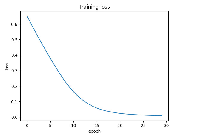
The final validation: run a full training loop on the GPU and plot the loss curve.
import torch.nn as nn
import torch.nn.functional as F
import matplotlib.pyplot as plt

device = "cuda" if torch.cuda.is_available() else "cpu"

model = nn.Sequential(
    nn.Linear(128, 256),
    nn.ReLU(),
    nn.Linear(256, 10)
).to(device)

optimizer = torch.optim.Adam(model.parameters(), lr=1e-3)

losses = []
for epoch in range(30):
    inp = torch.randn(32, 128, device=device)
    labels = torch.randint(0, 10, (32,), device=device)

    logits = model(inp)
    loss = F.cross_entropy(logits, labels)

    optimizer.zero_grad()
    loss.backward()
    optimizer.step()

    losses.append(loss.item())

plt.plot(losses)
plt.xlabel("epoch")
plt.ylabel("loss")
plt.title("Training loss")
plt.show()
This is the most important cell — it tests the entire ML training pipeline. If you’re new to machine learning, here’s what’s happening step by step:
What is a model?
A model is a mathematical function with adjustable parameters (called weights). You feed it input data, it produces a prediction, and then you adjust the weights to make the prediction better. Repeat this thousands of times and the model “learns” patterns in the data.
The model architecture
model = nn.Sequential(
    nn.Linear(128, 256),
    nn.ReLU(),
    nn.Linear(256, 10)
)
This defines a simple neural network with three layers:
-
nn.Linear(128, 256)— a fully connected layer. It takes an input of 128 numbers and multiplies it by a 128x256 matrix of learnable weights, producing 256 output numbers. Think of it like this: if each of the 128 input numbers represents a feature of a malware sample (e.g., file size, number of imports, entropy of sections, API call counts), this layer combines them all into 256 new values that capture more abstract patterns. This layer alone has 128x256 + 256 = 33,024 learnable parameters. -
nn.ReLU()— Rectified Linear Unit. A simple function: if a number is negative, replace it with zero; if positive, keep it as-is. This seems trivial, but it’s critical — without it, stacking multipleLinearlayers would be mathematically equivalent to a single linear transformation. ReLU introduces non-linearity, letting the network learn complex, non-linear patterns (like “if entropy is high AND import count is low, it’s more likely packed malware”). -
nn.Linear(256, 10)— the output layer. Maps 256 values down to 10, one for each class. In a real malware classifier, these 10 outputs might represent 10 malware families, and the highest value indicates the model’s prediction.
.to(device) moves all 33K+ parameters to the GPU so computation runs there.
The optimizer
optimizer = torch.optim.Adam(model.parameters(), lr=1e-3)
What is an optimizer? After the model makes a (probably wrong) prediction, we need to figure out how to adjust each of the 33K weights to make the prediction less wrong next time. The optimizer handles this automatically.
Adam (Adaptive Moment Estimation) is one of the most popular optimizers. It tracks a running average of recent gradients for each parameter and adapts the learning rate individually — parameters that need big updates get them, and parameters that are already close to optimal get smaller nudges. This generally converges faster than simpler approaches.
lr=1e-3 (0.001) is the learning rate — how big each adjustment step is. Too large and the model overshoots; too small and training takes forever. 0.001 is a common starting point.
The training loop
Each iteration (“epoch”) of the loop does four things:
1. Generate data:
inp = torch.randn(32, 128, device=device)
labels = torch.randint(0, 10, (32,), device=device)
Creates a batch of 32 fake samples, each with 128 features, plus 32 random class labels (0-9). In real malware detection, inp would be feature vectors extracted from executables (e.g., byte n-gram frequencies, behavioral API call sequences, PE header statistics) and labels would be ground-truth family labels from a labeled dataset.
2. Forward pass:
logits = model(inp)
loss = F.cross_entropy(logits, labels)
Feed the data through the model to get predictions (logits — raw scores for each class). Then measure how wrong the predictions are using cross-entropy loss. Cross-entropy is the standard loss function for classification: it compares the model’s predicted probability distribution across classes against the true label. A perfect prediction gives loss ≈ 0; a random guess on 10 classes gives loss ≈ 2.3 (which is ln(10)).
3. Backward pass (backpropagation):
optimizer.zero_grad()
loss.backward()
This is where the learning happens. loss.backward() computes the gradient of the loss with respect to every single parameter in the model — that’s 33K partial derivatives, calculated automatically using the chain rule from calculus. The gradient tells us: “if I increase this particular weight by a tiny amount, how much does the loss increase or decrease?” zero_grad() clears gradients from the previous iteration (PyTorch accumulates them by default).
4. Update weights:
optimizer.step()
The optimizer uses the gradients to nudge each weight in the direction that reduces the loss. After 30 epochs of this, the model has adjusted its weights enough to fit the training data.
Why the loss decreases
Looking at the plot, the loss drops smoothly from ~0.65 to near zero over 30 epochs. Even though the data is completely random, the model has enough capacity (33K+ parameters) to memorize the mapping from just 32 inputs to 32 labels. This is technically overfitting — the model is memorizing rather than generalizing.
That’s fine here. The point isn’t to build a useful model; it’s to confirm that every piece of the pipeline works: tensors move to the GPU, the forward pass runs, gradients flow backward, and the optimizer updates weights in the right direction. If any of these steps were broken, the loss would stay flat or explode.
Cell 8 — Generate Toy Behavioral Dataset
Now that the ML pipeline is validated with random data, let’s generate something closer to what a real malware detection experiment would use: behavioral API call sequences.
In dynamic malware analysis, a sandbox (like Cuckoo, CAPE, or Any.Run) executes a sample and records every Windows API call it makes. The sequence of API calls reveals what the program is actually doing — reading files, connecting to the network, injecting code into other processes, etc. This behavioral trace is one of the most powerful features for ML-based malware detection because it captures intent, not just static properties.
import random, json
random.seed(0)

benign = [
    ["CreateFileW","ReadFile","CloseHandle","RegOpenKeyExW","RegQueryValueExW","CloseHandle"],
    ["InternetOpenW","InternetConnectW","HttpOpenRequestW","HttpSendRequestW","InternetCloseHandle"],
    ["GetFileAttributesW","CreateFileW","WriteFile","FlushFileBuffers","CloseHandle"],
    ["CoInitializeEx","CoCreateInstance","RegOpenKeyExW","RegSetValueExW","RegCloseKey","CoUninitialize"],
]

malware = [
    ["VirtualAlloc","WriteProcessMemory","CreateRemoteThread","WaitForSingleObject","CloseHandle"],
    ["OpenProcess","VirtualAllocEx","WriteProcessMemory","GetThreadContext","SetThreadContext","ResumeThread"],
    ["NtAllocateVirtualMemory","NtWriteVirtualMemory","NtProtectVirtualMemory","NtCreateThreadEx","NtResumeThread"],
    ["CreateToolhelp32Snapshot","Process32FirstW","Process32NextW","OpenProcess","CreateRemoteThread"],
]

rows = []
for _ in range(80):
    rows.append({"label": "benign", "apis": random.choice(benign)})
    rows.append({"label": "malware", "apis": random.choice(malware)})

random.shuffle(rows)
print("rows:", len(rows))
This generates 160 samples (80 benign, 80 malware) — a small, balanced dataset for testing.
Understanding the API sequences
Benign patterns — these represent normal Windows application behavior:
CreateFileW → ReadFile → CloseHandle— opening, reading, and closing a file. Standard file I/O that any application performs.InternetOpenW → InternetConnectW → HttpOpenRequestW → HttpSendRequestW— WinINet API calls for making an HTTP request. Browsers, updaters, and legitimate apps use this all the time.RegOpenKeyExW → RegSetValueExW → RegCloseKey— reading or writing registry keys. Installers and configuration tools do this routinely.CoInitializeEx → CoCreateInstance— initializing COM objects. Standard Windows programming for interacting with system services.
Malware patterns — these represent process injection techniques commonly seen in real malware:
VirtualAlloc → WriteProcessMemory → CreateRemoteThread— classic DLL injection. The malware allocates memory in a remote process, writes shellcode or a DLL path into it, then creates a thread in that process to execute it. This is one of the most common injection techniques seen in trojans and RATs.OpenProcess → VirtualAllocEx → WriteProcessMemory → GetThreadContext → SetThreadContext → ResumeThread— thread context hijacking. Instead of creating a new thread, the malware suspends an existing thread in the target process, modifies its instruction pointer to point at injected code, then resumes it. Harder to detect thanCreateRemoteThread.NtAllocateVirtualMemory → NtWriteVirtualMemory → NtProtectVirtualMemory → NtCreateThreadEx— direct syscall injection. Uses the lower-levelNt*APIs from ntdll.dll instead of the higher-level kernel32.dll wrappers. Malware does this to bypass API hooking by security products that only monitor the kernel32 layer.CreateToolhelp32Snapshot → Process32FirstW → Process32NextW → OpenProcess → CreateRemoteThread— process enumeration followed by injection. The malware first lists all running processes (looking for a target likeexplorer.exeorsvchost.exe), then injects into the chosen one.
Why this matters
In a real ML pipeline, each sample would be an API trace from a sandbox run, and the model would learn to distinguish these patterns. The key insight is that benign software rarely needs to allocate memory in other processes or manipulate thread contexts — so even a simple model can learn to spot injection patterns.
This is a toy dataset with only 4 patterns per class, but the structure is identical to what we’ll use with real sandbox data later. The next step would be to convert these API sequences into numerical feature vectors (using techniques like bag-of-words, n-grams, or embeddings) and feed them to a model.
Result
All cells passed:
- Python and NumPy are functional on
aarch64 - PyTorch detects CUDA and the Jetson’s integrated GPU
- Tensor allocation and matrix multiplication work directly on GPU memory
- GPU benchmarking shows correct async/sync behavior
- A full training loop (forward pass, loss, backprop, optimizer step) completes with decreasing loss
- Behavioral API dataset generation works, ready for real feature engineering
The Jetson ML environment is ready for real experiments.